
by: Gad Mohamed
20/9/2020
Leave one out cross validation 8
Model evaluation on test set 9
K-nearest-neighbor (KNN) is a supervised machine learning algorithm that solves classification and regression problems. Despite being a supervised algorithm, KNN does not need training or learning a mapping function, instead, it relies on case-dependent predefined parameters to match the query data point to the “closest” training data point [1]. KNN parameters are:
Distance function. The distance metric used to compare the features of two data points. For each query point, KNN applies this function n times between the query point and each other data point in the training set. With n equals the number of data points in the training set.
K value. After comparing the query point to all points in the training set, and sort training set points ascendingly from the closest to the farthest, K is the number of closest neighbors to consider their votes in query evaluation, K is usually chosen as an odd number to have a tiebreaker.
Both KNN parameters are chosen, empirically, based on how the data features in concern respond to parameters variations. However, there are minimal assumption that must be met to ensure KNN is the right algorithm to use on data:
Feature importance are contained within its value. KNN, blindly, applies the distance function on features i.e. it does not weight features. Consequently, to give KNN a sense of the relative importance of each feature, features values should also represent the importance of the feature. More on that in data preprocessing section.
Relatively small Dataset. It is well known in machine learning algorithms that the smaller the dataset, the lower the performance. However, since KNN doesn’t learn a function from the data and needs to, iteratively, check each sample for each new query, a major setback in KNN is the high computational time or more precisely, the dependence of computational time on dataset size. i.e. the running complexity of KNN is O(kn + dn) for n is the dataset size, d is the vector dimension, and k is the K value. However, complexity changes depending on the implementation. For example, if instead of iterating k times to choose the lowest k distances we sort the distances, the complexity becomes O(nlong(n) + dn) ≈ O(n*log(n)).
Descriptive separable features. Raw features my represent a data point, but they do not always characterize it. Figure 1 shows samples from a face recognition task. Using KNN in that problem will be as accurate as random guessing since raw pixel values are low-level representation while we want features that encode the high-level information like hair style, skin tone, etc.… Needless to say, face recognition is an extreme example because face features are much more complicated than the MNIST features in hand, but the general idea here is, KNN assumes that the features on which the distance function is applied must directly describe not only the data, but the differences we are targeting within the data.

Figure 1 Raw features (pixel values) does not describe high-level aspects of a face. Source [2]
I started working by creating a quick baseline to assess each step I manipulate the data by comparing the result with the baseline performance. Fig 2. (a) shows the baseline performance on the normal MNIST and (b) shows the performance on the given noisy MNIST. Clearly, data preprocessing the data is crucial in this task. How to systematically approach the data? Each point considered in the aforementioned KNN assumptions will steadily boost performance or speed up the algorithm a bit.
In accordance with the first assumption, median filter is used to remove noise. Also, although binarizing the image make it seem clearer, we must not binarize the image because it’s important to give preserve the different values of pixels since they indicate the importance of the pixel to the classification of the image. For example, the low pixel values in the edge of a digit will have a lower weight – thus less important - in the distance than the pixel in the center of the digit. Fig. 2 shows the data before and after denoising as well as binarization effect on images.
Note: some parts of the digits have been erased due to binarization. However, this is not our focus here as this can easily be fixed using lower binarization threshold, our concern here is that all pixels in the binary image will either be on or off which means we loss the information of the relative importance of each pixel, which is given through different “on” values between edge and center of the digit.
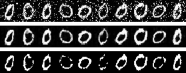
Figure 2 Top row: raw noisy images. Middle row: denoised using median filter (kernel size = 3). Bottom row: denoised and binarized images (degrades performance because it losses information _ pixels importance)
A smart move to reduce size as well as to better align data vectors for pixel-wise comparison, thereafter, is to crop images by removing all zero pixels in the four edges. Fig. 3 shows samples before and after cropping.
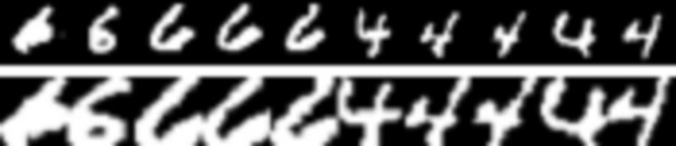
Figure 3Top row: samples before applying cropping. Bottom row: samples after applying cropping
Back in the “descriptive separable features” assumption we presented the problem of face
recognition, now we discuss the solution. Although face recognition state-of-art methods today are deep learning based relying on architectures like the Siamese network, a decent and cheap approach [3] is to convert the raw low-level features (pixels) of the image to high-level features (principle components) using dimensionality reduction tools like principle components analysis (PCA) or singular value decomposition (SVD). The key word here is variance. Dimensionality reduction tools will compute the covariance matrix of the data and choose the most P variant dimensions. Now instead of useless pixels, each new dimension is a weighted combination of pixels presenting a high-level feature [4]. P, the number of principle components, is another parameter added to our list.
The value of P which yields the highest model accuracy is 50 (compared to 28*28=784) which also resulted in speeding up the algorithm. However, Fig. 4 shows the plot of sample of data of different labels (denoted with different point color) in a 3D space after using P value of 3. This also gives us an idea on how much “separable” our data is.

Figure 4 a 3D plot of images with different labels using P value = 3. we can identify clusters of points having the same color (representing the same class)
KNN is relatively easy to implement. I designed the code with modularity in mind so that I can define different distance and preprocessing functions and, easily, try different combination of them and compare performance.
After choosing the adequate parameters (k value, p value, distance function, …) and the best combination of preprocessing functions, I re-ran the baseline model and compared my implementation to the baseline in terms of accuracy and speed. I found my model to be slightly worse in terms of both accuracy and speed.
Regarding the accuracy, I think the problem might be in the distance function since I use the standard Euclidean metric while sklearn’s KNN [1] default distance function is ‘minkowski’. Regarding speed, I mentioned earlier the complexity of KNN and how it is affected by using
sorting or just iterating K times. Since I use soring (as suggested in the task description), it is justified that my implementation will be slightly slower.
KNN parameters as well as number of principle components are chosen empirically. I
have, iteratively, tried the principle components values range from 3 to 600 (default is 28*28=784) and K values range from 1 to 15. I have also tried custom and off-shelf distance functions like Euclidean and mean absolute error (MAE).

Figure 5 model accuracy response to different K & P values. The best K value, regardless of the P value, is 1
In the file named my_KNN_LOOCV.py I apply the leave one out validation algorithm on my implementation of KNN. Using P value of 42 and K value range from 1 to 101 (with step size: 2 to have a tiebreaker). Worth noting here that the P value of 42 compared to the raw features size of 28*28=784 significantly reduced size and increased speed.
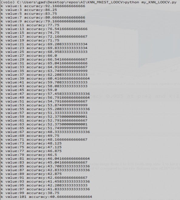
Figure 6 leave-one-out cross validation using P value of 42 and K values range from 1 to 101 with step size 2
Thus, we learn that the optimal values for P and K are 42 and 1, respectively.
In my_KNN_test.py I tested my KNN implementation on test set and got 93.5% as shown in the following image, using the optimal values for P and K which are 42 and 1, respectively.

Figure 7 Model accuracy (correct/total) on the test set
Confusion matrix is a statistical analysis tool to assess the performance of the model. Since terms like true positives (TP), true negatives (TN), false positives (FP), and false negatives (FN) usually refer to binary classification, in multi class classification, the confusion matrix is used instead. The diagonal of the matrix shows the correctly predicted classes while all other cells presents deviations or FNs.
The figure below shows confusion matrices of my implementation of KNN on test set. The confusion matrix on the left is built by me while the confusion matrix on the right is built using seaborn visualization library.
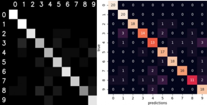
Figure 8 LEFT: confusion matrix of testset built by me. RIGHT: confusion matrix of testset constructed by seaborn
In the report I presented my work of classification a noisy MNIST handwritten digits data set using KNN. I have explored different preprocessing, and distance functions as well as dimensionality reduction tools all to meet the assumption on which KNN operates.
The question of whether this problem is suitable for KNN is also a question of whether it is possible to fulfil KNN’s assumptions to a reasonable extent. Judging on the results we got (93.5% on test set), I think KNN is suitable for such a medium-sized easy- to-interpret data.
However, since MNIST dataset is available with much more data, a deep learning based method will yield a better result. In fact, Yann Lecun, maintains a 70000 sized MNIST dataset with a collection of classification methods from 1998 to 2012 and test error rate ranging from 12% to 0.23 (88% to 99.77% accuracy). The list clearly shows deep learning based methods dominating the highest performance methods [5].
sklearn.neighbors.KNeighborsClassifier — scikit-learn 0.23.2 documentation. Scikit-learn.org. (2020).
Retrieved 21 September 2020, from https://scikit- learn.org/stable/modules/generated/sklearn.neighbors.KNeighborsClassifier.html.
kutz, n. (2020). Data-Driven Modeling & Scientific Computation: Methods for Complex Systems & Big Data (2nd ed.). Oxford University Press.
gad, g. (2020). gadm21/Face-recognition-using-PCA-and-SVD. GitHub. Retrieved 21 September 2020, from https://github.com/gadm21/Face-recognition-using-PCA-and-SVD.
A One-Stop Shop for Principal Component Analysis. Medium. (2020). Retrieved 21 September 2020, from https://towardsdatascience.com/a-one-stop-shop-for-principal-component-analysis-5582fb7e0a9c.
MNIST handwritten digit database, Yann LeCun, Corinna Cortes and Chris Burges. Yann.lecun.com. (2020). Retrieved 21 September 2020, from http://yann.lecun.com/exdb/mnist/.