Next: Bibliography Up: Efficient implementation Previous: Efficient implementation
 be a primitive
  .
We define
.
We define
![\begin{displaymath}\begin{array}{rcl} A^{[0]}(x) & = & a_0 + a_2 x + a_4 x^2 + \...
... + a_3 x + a_5 x^2 + \cdots + a_{n-1} x^{n/2 -1} \\ \end{array}\end{displaymath}](img329.png) |
(55) |
![$\displaystyle A(x) \ = \ A^{[0]}(x^2) + x \, A^{[1]}(x^2).$](img330.png) |
(56) |
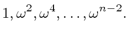
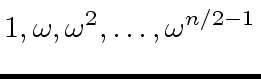
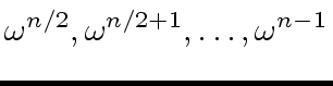
 is reduced to evaluate
  .
But this second sequence of powers of
.
But this second sequence of powers of  .
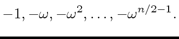
Indeed, for every integer
.
Indeed, for every integer 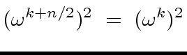 |
(57) |
 holds, we obtain
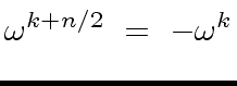 |
(58) |
 |
(59) |
 |
(60) |
 |
(61) |
 |
(62) |
 we have
The validity of Algorithm 3 follows from the two following observations.
 ,
then
,
then
 defines
an ordering of the coefficients of
defines
an ordering of the coefficients of
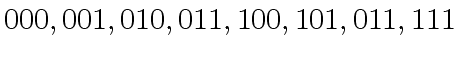
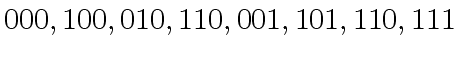
Observe that if the input array ![]() is sorted w.r.t. this
DFT ordering, one can describe easily the
recursive calls with a binary tree.
If this tree is traversed bottom-up, from left to right,
we are led to an iterative algorithm working in place!
For instance, for
is sorted w.r.t. this
DFT ordering, one can describe easily the
recursive calls with a binary tree.
If this tree is traversed bottom-up, from left to right,
we are led to an iterative algorithm working in place!
For instance, for ![]() , assuming that the input array
, assuming that the input array ![]() is
is
 |


![$ [a_0, a_4, a_2, a_6, a_1, a_5, a_3, a_7]$](img374.png) ,
observe that this ordering changes
,
observe that this ordering changes
 |
(64) |
 |
(65) |
![$ {\mbox{${\mathbb{Z}}$}}[x]$](img377.png) .
We can assume that all their coefficients are positive.
Otherwise, we can restrict to this case by setting
.
We can assume that all their coefficients are positive.
Otherwise, we can restrict to this case by setting
 |
(66) |
 |
(67) |
 ,
,
 ,
,  and
and  one after another.
 and
and
 be the max-norms of
  |
(68) |
 be primes such
 is bigger than
 ![$ {\mbox{${\mathbb{Z}}$}}/p_i{\mbox{${\mathbb{Z}}$}}[x]$](img399.png) using the FFT-based multiplication.
using the FFT-based multiplication.
Marc Moreno Maza
![\begin{displaymath}\begin{array}{rcl} A({\omega}^i) & = & A^{[0]}({\omega}^{2i})...
...ga}^{2i}) - {\omega}^i \, A^{[1]}({\omega}^{2i}) \\ \end{array}\end{displaymath}](img343.png)
![\fbox{
\begin{minipage}{10 cm}
\begin{description}
\item[{\bf Input:}] $n = 2^r$...
...n/2}$\ := $y_k^{[0]} - t$\ \\
\> {\bf return} $y$
\end{tabbing}\end{minipage}}](img344.png)
![\begin{figure}\htmlimage
\centering
\includegraphics[scale=.5]{fft8.eps}\end{figure}](img372.png)
![\fbox{
\begin{minipage}{12 cm}
\begin{description}
\item[{\bf Input:}] $n = 2^r$...
...k + j + m/2]$\ := $u - t$\ \\
\> {\bf return} $A$
\end{tabbing}\end{minipage}}](img373.png)