Proof.
Clearly the polynomial
f of Relation (
31)
satisfies Relation (
30).
Hence the existence is clear.
The unicity follows from the fact that the difference of
two such polynomials has
- degree less than n and
- n roots
hence is the zero polynomial.

Proof.
We saw in Remark
7 that evaluating the polynomial
f
of degree
n at one point costs 2
n - 2 operations in

.
So evaluating
f at
u0,...,
un-1 amounts to
2
n2 - 2
n.
Let us prove now that interpolating a polynomial at
u0,...,
un-1 can be done in

(
n2) operations in

.
We first need to estimate the cost of computing the
i-th interpolant
Li(
u).
Consider
m0m1,
m0m1m2, ...
m =
m0 ... mn-1
where
mi is the monic polynomial
mi =
x -
ui.
Let
pi =
m0m1 ... mi-1 and
qi =
m/
mi for
i = 1
... n.
We have
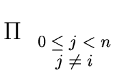
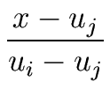
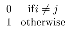
Li(u) =  |
(32) |
To estimate the cost of computing the
Li(
u)'s let us start with that of
m.
Computing the product of the monic polynomial
pi =
m0m1 ... mi-1 of degree
i
by the monic polynomial
mi =
x-ui of degree 1 costs
- i multiplications (in the field
 ) to get
- ui pi plus
- i - 1 additions (in the field
 ) to add
- ui pi (of degree i)
to x pi (of degree i + 1 but without constant term)
leading to
2
i - 1.
Hence computing
p2,...,
pn =
m amounts to
 2 i - 1 2 i - 1 |
= |
 2 i + 1 2 i + 1 |
| |
= |
2 i + n - 1 i + n - 1 |
| |
= |
2 n (n - 1)/2 + n - 1 |
| |
= |
(n - 1)(n + 1) |
|
(33) |
Computing
qi implies a
division-with-remainder of the polynomial
m of degree
n by the polynomial
mi of degree 1.
This division will have
n - 1 + 1 steps, each step requiring 2 operations
in

.
Hence computing all
qi's amounts to
n 2
n.
Since
qi has degree
n - 1 computing each
qi(
ui)'s
amounts to 2
n - 2 operations in the base field

(from Remark
7).
Then computing all
qi(
ui)'s amounts to
2
n2 - 2
n.
Then computing each
Li(
u) =
qi/
qi(
ui) from the
qi's and
qi(
ui)'s costs
n.
Therefore computing all
Li(
u)'s from scratch
amounts to
(
n - 1)(
n + 1) + 2
n2 + 2
n2 - 2
n +
n2 = 6
n2 - 2
n - 1.
Computing f from the Li(u)'s requires
- to multiply each Li(u) (which is a polynomial of degree n - 1) by the number vi
leading to n2 operations in
 and
and
- to add these
vi Li(u) leading to n - 1 additions
of polynomials of degree at most n - 1
costing (n - 1)n operations in

amounting to
2
n2 -
n.
Finally the total cost is
6
n2 - 2
n - 1 + 2
n2 -
n = 8
n2 - 3
n - 1

![]() be a field and let
u = (u0,..., un-1)
be a sequence of pairwise distinct elements of
be a field and let
u = (u0,..., un-1)
be a sequence of pairwise distinct elements of ![]() .
.


