Proof.
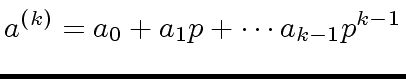
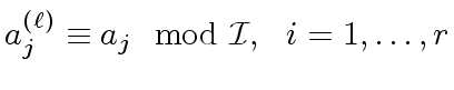
Let
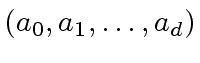
be a

-adic expansion of

w.r.t.
.
Let
be a positive integer.
By Proposition
6,
the element
 |
(12) |
is a
-adic approximation of
at order

.
By Proposition
4
there exists a polynomial
![$ {\psi} \in R[y]$](img83.png)
such that
 |
(13) |
Since we have
we deduce from Proposition
7
 |
(14) |
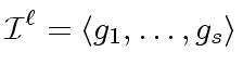
Since
this shows that
is in the ideal generated by

.
Similarly,
is in the ideal generated by

.
Therefore we can divide
and
by
, leading to
 |
(15) |
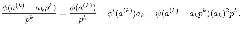
Now observe that
 |
(16) |
Let us denote by

the canonical homomorphism from

to

.
Then we obtain
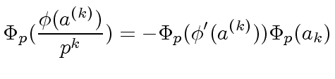 |
(17) |
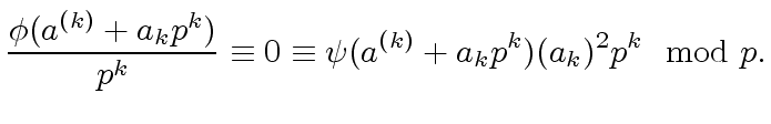
Now, since
holds we have
 |
(18) |
Since
holds we can solve
Equatiion
17
for

.
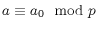
Finally, from Theorem
1,
we have
such that we can
view
as

. This is straightforward if

or if
![$ R = {\bf k}[x]$](img138.png)
where

is a field, since we can choose for

the remainder of

modulo
.

Proof.
We proceed by induction on

.
For

the claim follows from the hypothesis of the theorem.
So let
be such that the claim is true.
Hence there exist
such that
 |
(20) |
and
 |
(21) |
Since

is finitely generated, then so is

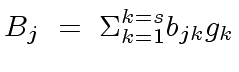
and let
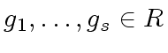
such that
 |
(22) |
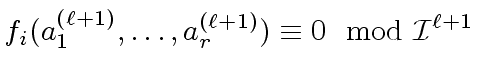
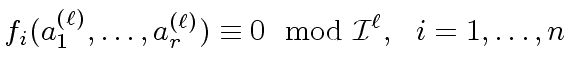
Therefore, for every
, there exist
such that
 |
(23) |
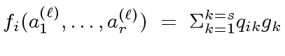
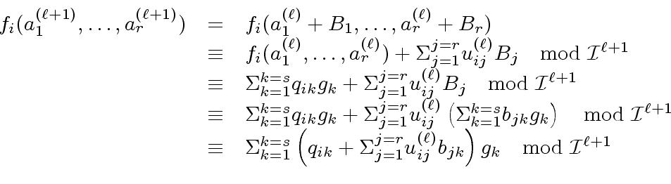
For each
we want to compute
such that
 |
(24) |
is the desired
next approximation.
We impose
so let
be such that
 |
(25) |
Using Proposition
5
we obtain
 |
(26) |
where

is the Jacobian matrix
of
at
.
Hence, solving for
 such that
leads to solving the system of linear equations:
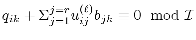 |
(27) |
for
and
.
Now using
 for
we obtain
for
we obtain
 |
(28) |
Therefore the linear system equations
given by Relation (
27)
has solutions.
 be a prime element.
Let
be a prime element.
Let
![$ {\phi} \in R[y]$](img64.png) and let
and let
 such that
![$ f_1, \ldots, f_n \in R[x_1, \ldots, x_r]$](img141.png) be
be  .
Let
.
Let
 be elements.
Let
be elements.
Let  evaluated at
 .
That is,
.
That is,  matrix defined by
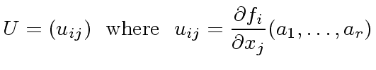
 .
.
 ,
,